
How TAWQ works
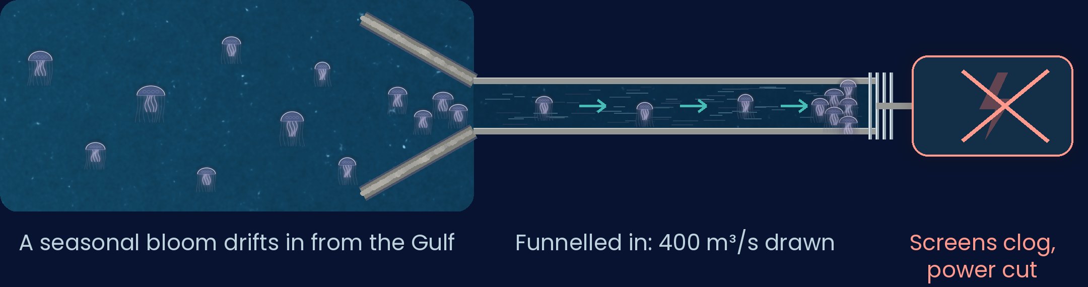
In shortA ring of bubbles far out at sea holds the jellyfish back, the air goes where the tide pushes water in, and robot boats carry the held jellyfish out to sea.
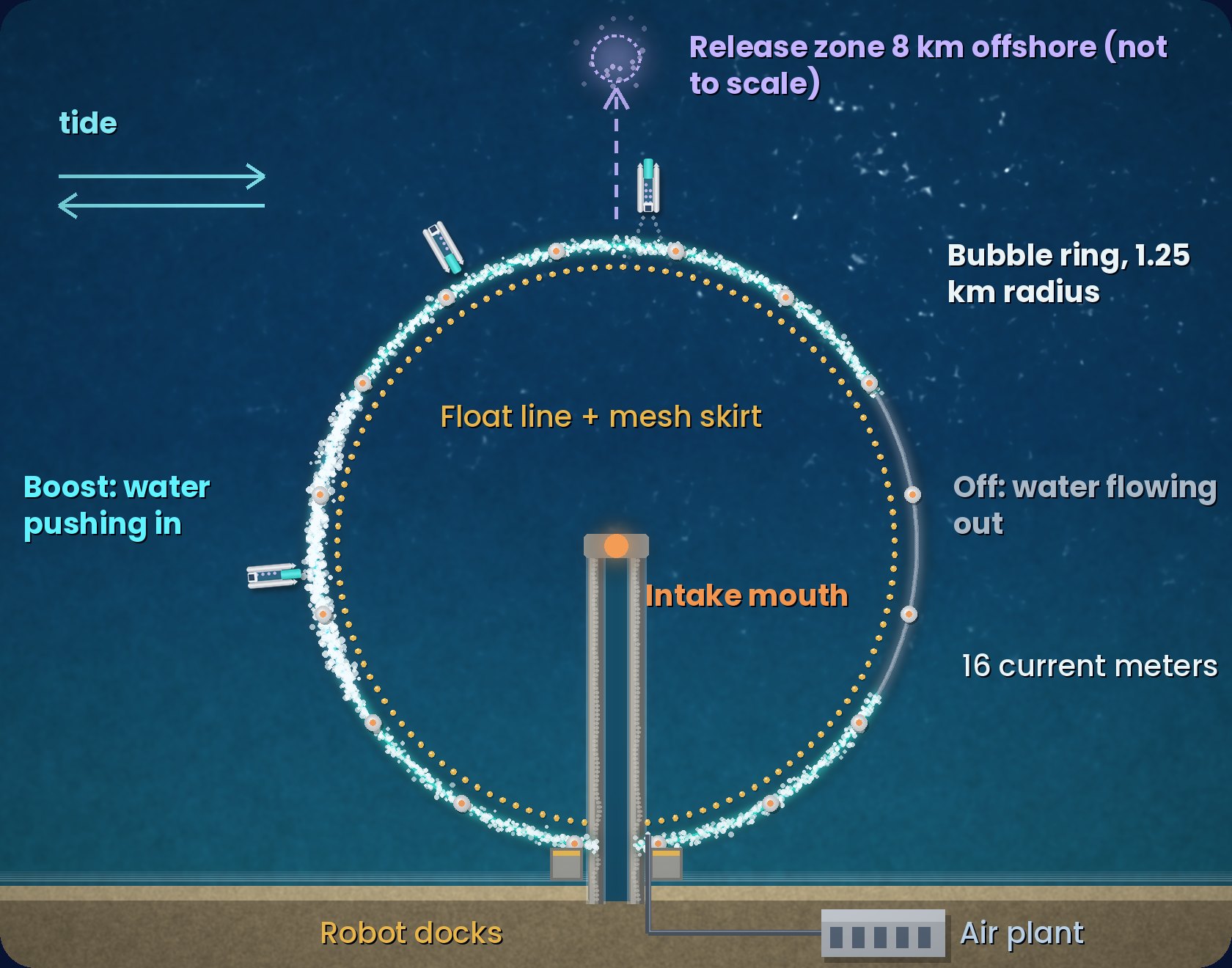
- Warning, air onThe early-warning notification switches the ring on before the bloom arrives.
- HoldRising bubbles from four seabed pipes turn most drifting jellyfish back; a float line with a mesh skirt keeps them in the band.
- Air follows the tide240 sections and 60 air valves: boosted where water pushes in, off where it flows out. If control is lost, the valves open and every section gets normal air.
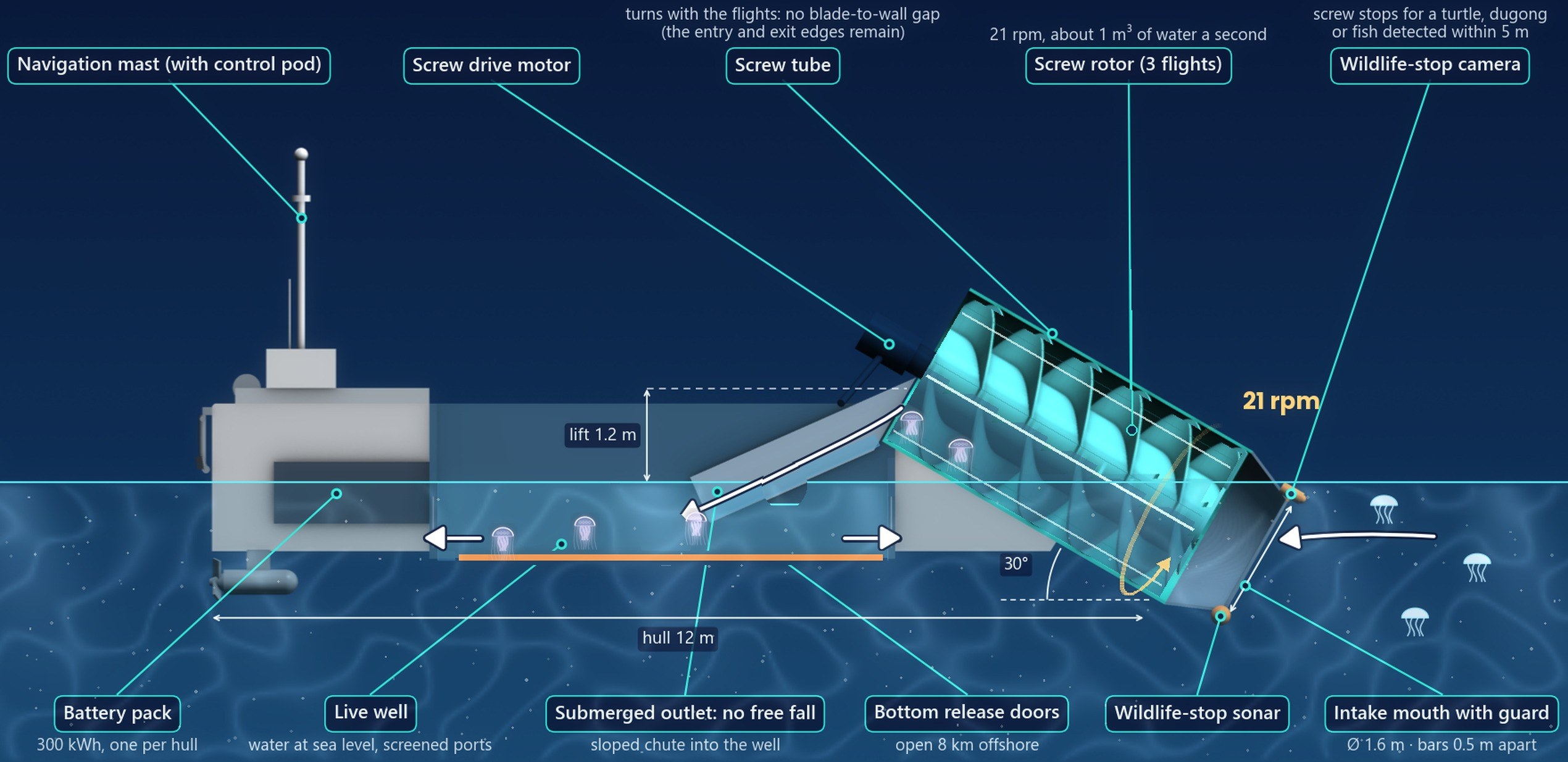
- LiftRobot catamarans lift the held jellyfish, in water, with a slow Archimedes screw into the live well. The screw stops if a turtle, dugong or fish is within 5 m. Designed for live handling; survival rates are measured in the Phase 0 trials.
- ReleaseThey carry them 8 km offshore and release them; in our model none drift back within 21 days.
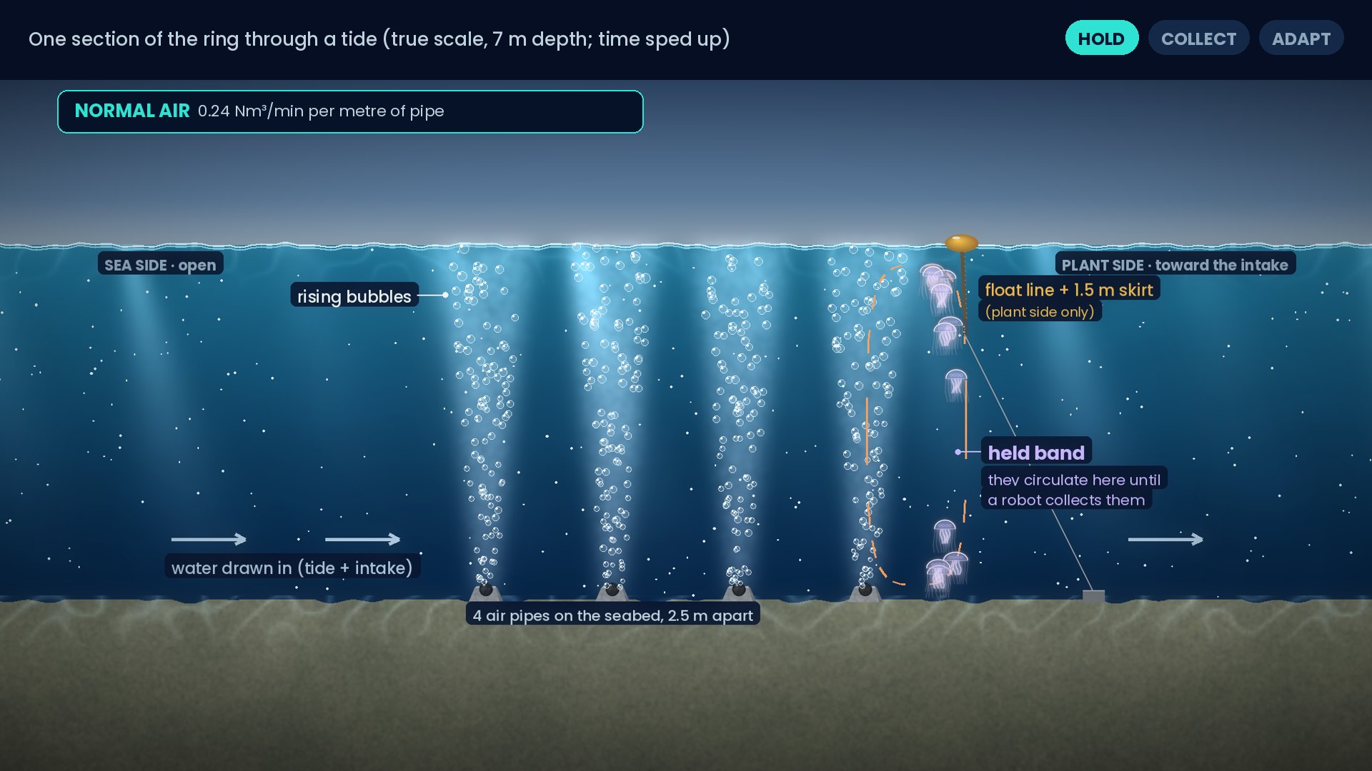
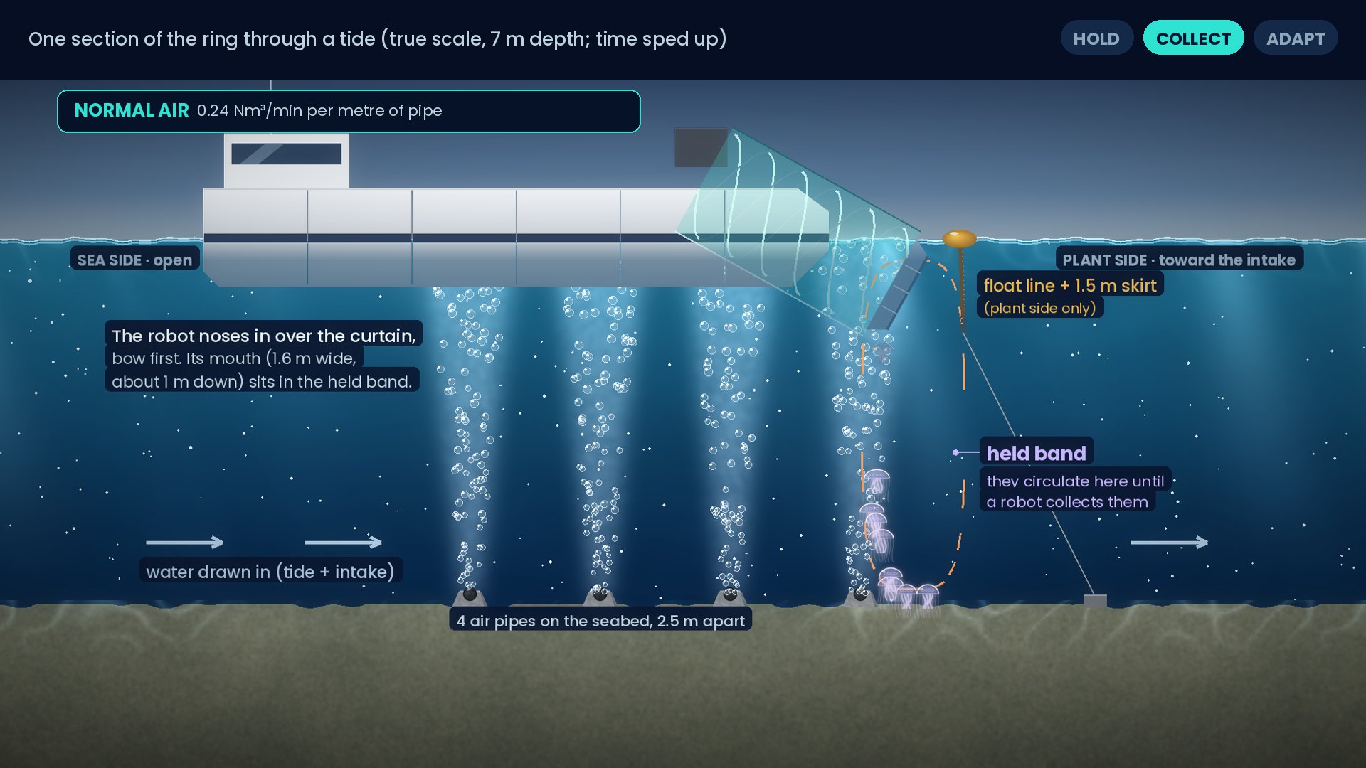
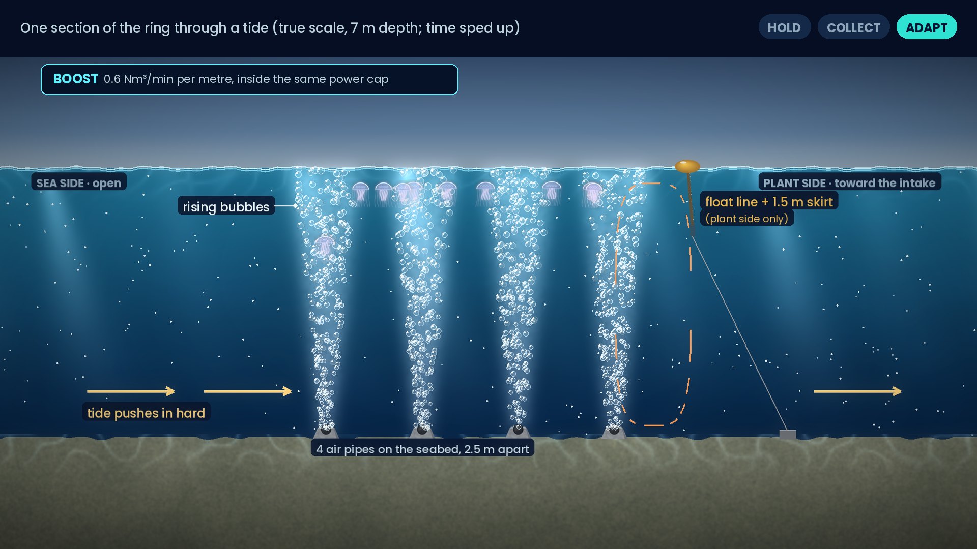
Why so far out? At the intake mouth the water moves at about 0.38 m/s (estimated), about three times the most a bubble curtain can hold (about 0.13 m/s). 1.25 km out, the intake's pull is only about 1.3 cm/s, so the tide decides which way the water moves. See the calculation.
Why it matters. ENEC asks, for the stage after an early-warning notification: “How might we advance the sustainable management of seasonal jellyfish blooms in coastal environments?” (ENEC 2026). At Gravelines, France, on 10–11 August 2025, jellyfish in the cooling-water filters shut down four reactor units (2, 3, 4 and 6) (AFP 2025).
The three models and how they connect
In shortThree linked computer models (the water around the site, the bubble curtain, and a 3‑day bloom) turn published site data and our stated assumptions into every result on this page.
Site flow model
A plan-view model of the water around the intake: the intake's pull, the tide and the breakwater arms.
- Inputs
- Intake flow 400 m³/s (bound 690); the site layout and seabed depth; four background-current cases.
- Produces
- Water speed everywhere, including the inward speed on each of the ring's 240 sections; the intake's pull at the ring, about 1.3 cm/s.
Curtain model
A 2D vertical slice through the bubble curtain: the rising plume drives a surface current, and drifting jellyfish either stay on the sea side or cross.
- Inputs
- Water depth; air per metre of pipe; inward water speed; a mesh skirt 10 % blocked; a 12‑hour hold.
- Produces
- The holding limit, the fastest inward current the curtain still holds against: 0.081–0.112 m/s with normal air, 0.085–0.126 m/s with boost.
3‑day bloom model
12,000 virtual jellyfish drift with the modelled water. At the ring each one is held, crosses or is pushed through; robots remove held jellyfish at the fleet's rate.
- Inputs
- Water speeds from the site model; holding limits from the curtain model, section by section; the air state from the tide-aware controller; a design bloom of 5 g/m³; the robot fleet's rate.
- Produces
- The share of the bloom reaching the intake, tonnes per day, the worst single hour, and the held stock.
How the results are sampled. Each configuration is run from 24 tide start times spread over one spring–neap cycle (14.77 days), with 12,000 virtual jellyfish each, in four background-current cases: one randomly varying current, the central case, with the measured spread of 4.8 cm/s; and three steady currents, 0, +0.05 and −0.05 m/s, as bounds. Every configuration starts from the same jellyfish positions in each tide start, so comparisons are like with like.
Supporting calculations. The air controller (which sections get boost or no air, and the power it needs), robot sizing (energy, charging, availability), a release model (where released jellyfish drift over 21 days in a 16 km area), the air supply and a cost model.
Species. ENEC's focus species is the Blue Blubber (Catostylus mosaicus). Our bloom model works in biomass (grams of jellyfish per cubic metre of water), so it does not depend on animal size.
Detailed calculations
In shortEvery number we quote, with how it was calculated and where each input comes from.
Rounding: each number is rounded once from the unrounded model value, half away from zero, to the precision used in our deck; the calculation panels may show one more digit. Each result is computed from unrounded values, so redoing a sum with the rounded inputs shown can differ in the last digit.
3.1 The site
Intake flow: 400 m³/s
The plant draws 400 m³/s of seawater for cooling; we also test 690 m³/s as a conservative bound.Show the calculationHide the calculation
flow = number of units × condenser flow per unit
| Input | Value | Source |
|---|---|---|
| Condenser cooling water per unit | 6,000 m³/min | Published ENEC 2017 |
| Reactor units | 4 | Published Power Engineering 2021 |
| Design maximum per unit (bound) | 172.5 m³/s | Published NEI 2012 |
| Flows used in the models | 400 and 690 m³/s | Model output master_params.json |
4 × 6,000 m³/min ÷ 60 s/min = 400 m³/s
Bound: 4 × 172.5 m³/s = 690 m³/s
This is the condenser cooling flow. The safety-related essential service water system takes Gulf seawater through its own “essential service water intake structure” (FANR 2012), so it is not part of this flow.
Water speed at the intake mouth: about 0.38 m/s
About 0.38 m/s (estimated: channel width fitted to NMDC's published dredged area). That is about three times the best holding limit of a bubble curtain, about 0.13 m/s (2.8–3.0×), so a curtain at the mouth would hold nothing.Show the calculationHide the calculation
speed = flow ÷ mouth area; mouth area = channel width × depth; ratio = speed ÷ best holding limit
| Input | Value | Source |
|---|---|---|
| Intake flow | 400 m³/s | Published ENEC 2017 |
| Channel width: one average width for the three dredged channels | 162 m | Model output final_numbers.json |
| Depth at the breakwater heads (breakwater toe) | 6.5 m | Our assumption inside NMDC's published channel depths of −5.5 to −9.5 m |
| Total dredged area of the three channels | 2.35 km² | Published NMDC |
| Length of the three channels | 14.50 km | Our assumption our estimate from the seabed profile (ETOPO 2022, not survey data); NMDC publishes no channel widths or lengths |
| Best holding limit (boost, deepest section) | 0.126 m/s | Model output system.json |
Width fit: 2.35 km² ÷ 14.50 km = 162 m
400 ÷ (162 × 6.5) = 400 ÷ 1,053 m² = 0.380 m/s → about 0.38 m/s
0.380 ÷ 0.126 = 3.0 times
NMDC publishes only the total dredged area, not channel widths, so the width is a fit. The same fit puts the intake channel at 7.0 m deep; with that depth the speed is 0.35 m/s and the ratio 2.8. Either way the mouth is far above what a curtain can hold.
The intake's pull at the ring: about 1.3 cm/s
About 1.3 cm/s at 1.25 km out: small next to the tide, so the tide decides which way the water moves at the ring.Show the calculationHide the calculation
pull at the ring = inward speed caused by the intake alone at the ring radius (site flow model)
| Input | Value | Source |
|---|---|---|
| Intake's pull at the ring | 1.32 cm/s | Model output final_numbers.json |
| Tide speed at the ring, typical (root mean square) | 4.6 cm/s | Model output final_numbers.json |
| Tide speed at the ring, peak | 11.7 cm/s | Model output final_numbers.json |
1.32 cm/s from the intake, against a typical 4.6 cm/s and a peak 11.7 cm/s from the tide.
3.2 Holding the bloom
Holding limits and the ×0.85 / ×0.76 factors
The curtain holds against inward water up to 0.081–0.112 m/s with normal air and 0.085–0.126 m/s with boost, depending on depth. These limits include factors of ×0.85 (normal air) and ×0.76 (boost) for a mesh skirt 10 % blocked and a 12‑hour hold.Show the calculationHide the calculation
holding limit = curtain-model limit (clean, short hold) × factor; factor = mesh effect × hold-time effect
| Input | Value | Source |
|---|---|---|
| Limit, clean curtain, 7 m deep, normal air 0.24 Nm³/min per m, 3.6 h hold | 0.1185 m/s | Model output slice_A.json |
| Same with the mesh skirt 10 % blocked | 0.1071 m/s | Model output slice_E.json |
| Mesh skirt, 3.6 h and 12 h hold | 0.1071 → 0.1010 m/s | Model output slice_I.json |
| Mesh skirt, boost air 0.6 Nm³/min per m, 3.6 h | 0.1333 m/s | Model output slice_H.json |
| Boost limit before the corrections, 7 m deep | 0.1664 m/s | Model output system.json |
| Mesh skirt blocked | 10 % | Our assumption fouling rate unknown; measured at the pilot section (step 2) |
| Hold-time basis | 12 h | Our assumption held jellyfish can stay at the curtain for many hours |
Normal air: mesh 0.1071 ÷ 0.1185 = 0.904; hold 0.1010 ÷ 0.1071 = 0.943; factor 0.904 × 0.943 = 0.852 → ×0.85
Boost: mesh 0.1333 ÷ 0.1664 = 0.801; factor 0.801 × 0.943 = 0.756 → ×0.76
Limits along the ring (shallowest to deepest section): normal 0.095–0.132 × 0.85 = 0.081–0.112 m/s; boost 0.112–0.166 × 0.76 = 0.085–0.126 m/s
The two factors were typed into the model as 0.85 and 0.76; they reproduce from the curtain-model runs above. With the mesh 40 % blocked the curtain model holds nothing (limit 0.00 m/s), so the mesh must be kept clean.
3.3 Air that follows the tide
- Off: water flowing out 18 %
- Normal air 76 %
- Boost: water pushing in hard 6 %
Share of section-time over a month of tides, all 240 sections, from the air-control model.
Held per crossing: 86.9 % against 80.4 %
With tide-aware air, 86.9 % of the jellyfish drifting in across the ring meet a section that can hold them at that crossing, against 80.4 % with fixed air. Before any robots, 6.9 % of a design bloom reaches the intake with tide-aware air, against 8.8 % with fixed air.Show the calculationHide the calculation
held share = inward water flux crossing where the speed is below the section's holding limit ÷ all inward flux across the ring. Jellyfish drift with the water, so this is the share of arriving jellyfish held per crossing.
| Input | Value | Source |
|---|---|---|
| Held per crossing, tide-aware / fixed air | 86.9 / 80.4 % | Model output system.json |
| Share of the bloom reaching the intake, tide-aware / fixed (central case) | 6.89 / 8.80 % | Model output summary.json |
Held per crossing explains the mechanism only; the share of the bloom reaching the intake is the result that counts.
Air power: 12 % less than fixed air
Tide-aware air uses 12 % less power: 12.8 MW on average against 14.6 MW for fixed air (design basis).Show the calculationHide the calculation
saving = 1 − tide-aware mean power ÷ fixed-air power
| Input | Value | Source |
|---|---|---|
| Tide-aware air, mean power | 12.82 MW | Model output system.json |
| Fixed air (every section at normal air) | 14.63 MW | Model output system.json |
1 − 12.82 ÷ 14.63 = 12.4 % → 12 % less
Fixed air runs every section at normal air all the time. That equals the cap the tide-aware controller never exceeds, so the comparison is like with like.
Running power: 14 MW, 0.25 % of the plant's output
The ring draws 14 MW on average while it is on: 0.25 % of the plant's 5,600 MW.Show the calculationHide the calculation
running power = air power × hot-inlet factor × aftercooler factor + main-pipe losses + aftercooler pumps
| Input | Value | Source |
|---|---|---|
| Tide-aware air power | 12.82 MW | Model output system.json |
| Hot-inlet factor | × 1.02 | Our assumption allowance for hot summer air at the blower inlet |
| Aftercooler pressure-drop factor | × 1.023 | Model output aftercooler.json (2.28 % extra power, rounded) |
| Main-pipe losses, deep / shallow | 0.328 / 0.175 MW | Model output air_supply.json |
| Aftercooler pumps | 0.171 MW | Model output aftercooler.json |
| Plant output, four units | 5,600 MW | Published Power Engineering 2021 |
12.82 × 1.02 × 1.023 + 0.328 + 0.175 + 0.171 = 14.0 MW
14.0 ÷ 5,600 = 0.251 % → 0.25 %
Energy: about 337 MWh a day for the air (345 with robot charging).
Blowers and aftercoolers
44 turbo blowers of 400 kW: 17.6 MW installed, including 2 spares. Seawater aftercoolers cool the air from up to 133 °C to 40 °C for the plastic pipe; their cooling water returns 5 °C warmer, 0.85 m³/s.Show the calculationHide the calculation
installed power = number of blowers × unit size
| Input | Value | Source |
|---|---|---|
| Blowers: deep only / shallow only / swing / spare | 26 / 12 / 4 / 2 | Model output cost2_r12.json |
| Peak demand, including losses | 16.8 MW | Model output cost2_r12.json |
| Air leaving the blowers in summer (45 °C inlet) | 133 °C | Model output aftercooler.json |
| Heat removed; seawater flow | 17.4 MW; 0.85 m³/s | Model output aftercooler.json |
44 × 400 kW = 17.6 MW
3.4 What reaches the intake
Share of a 3‑day design bloom reaching the intake. Bar: central case. Whisker: range over all four current cases. 24 tide starts × 12,000 virtual jellyfish. The mouth bar is set equal to doing nothing by argument, not by a model run.
LimitThe ring cuts the total load, not the worst hour: in the central case the average worst hour is about the same (12.1 vs 12.2 t/h) and the single worst hour about doubles (36.1 vs 18.1 t/h). In 17 of 96 tide-start cases the worst hour is above doing nothing.
75 % less reaches the intake; 73 → 18 t/day
With the ring and 12 robots, 3.8 % of a 3‑day design bloom reaches the intake, against 15.3 % with no ring: 75 % less in the central case (about ±8 points, 2 standard errors over 24 tide starts). The load on the screens falls from 73 to 18 t/day.Show the calculationHide the calculation
reduction = 1 − (intake with the ring) ÷ (intake with no ring), both summed over the 24 tide starts
| Input | Value | Source |
|---|---|---|
| Share reaching the intake, no ring | 15.33 % | Model output summary.json |
| Share reaching the intake, ring + 12 robots | 3.79 % | Model output summary.json |
| Load on the screens, no ring / ring + 12 robots | 72.9 / 18.0 t/day | Model output summary.json |
| Design bloom | 5 g/m³: 1,426 t within 4 km (the deck rounds it to about 1,400 t) | Our assumption no published Gulf biomass density was found |
| Sampling | 24 starts × 12,000 jellyfish | Our assumption design choice |
1 − 3.79 ÷ 15.33 = 75.3 % → 75 %
72.9 → 18.0 t/day → 73 → 18 t/day
The same jellyfish start positions are used for every configuration in each tide start, so the comparison is paired.
Every configuration and current case
Under steady currents the ring + 12 robots cut the share reaching the intake by 71–97 %; the table shows all 7 configurations in all four current cases.Show the calculationHide the calculation
Swipe sideways to see the whole table.
| Configuration | Central | Steady 0 | Steady +0.05 | Steady −0.05 |
|---|---|---|---|---|
| No ring | 15.3 % | 21.7 % | 12.6 % | 12.1 % |
| Ring, fixed air | 8.8 % (43 %) | 2.7 % (87 %) | 5.2 % (59 %) | 7.7 % (36 %) |
| Ring, tide-aware air | 6.9 % (55 %) | 1.0 % (95 %) | 4.2 % (67 %) | 6.7 % (44 %) |
| Ring + 6 robots | 5.1 % (67 %) | 0.7 % (97 %) | 3.7 % (71 %) | 4.4 % (64 %) |
| Ring + 8 robots | 4.5 % (71 %) | 0.7 % (97 %) | 3.6 % (72 %) | 3.9 % (67 %) |
| Ring + 10 robots | 4.2 % (73 %) | 0.7 % (97 %) | 3.5 % (72 %) | 3.8 % (69 %) |
| Ring + 12 robots | 3.8 % (75 %) | 0.7 % (97 %) | 3.5 % (72 %) | 3.5 % (71 %) |
Share of the design bloom reaching the intake; in brackets, the reduction against no ring. Central = randomly varying current; steady currents in m/s. Model output summary.json
Ring + 12 robots under steady currents of 0, +0.05 and −0.05 m/s: 96.9 %, 72.2 % and 70.9 % → 71–97 %
Reduction against no ring. Central case: about ±8 points (2 standard errors over 24 tide starts). All cases except the steady currents use the central (randomly varying) current. The meters case replaces the model's full knowledge of the current with current meters and a tide forecast.
Bound cases: Shamal wind, offshore wind, 690 m³/s
In a steady 10 m/s Shamal wind the cut is 56 %; with a steady offshore wind 86 %; with the intake at its design maximum of 690 m³/s, 72 %. At 690 m³/s the worst hour is the weak point: it is above doing nothing in 13 of 24 tide starts (mean worst hour 27.3 vs 18.3 t/h).Show the calculationHide the calculation
| Input | Value | Source |
|---|---|---|
| Reduction, Shamal wind (central current) | 55.5 % | Model output summary_wind_se.json |
| Reduction, offshore wind | 86 % | Model output summary_wind_n.json |
| Reduction, 690 m³/s | 72 % | Model output summary_q690.json |
| Shamal case: a steady wind driving surface water toward the coast | 10 m/s | Our assumption a test case; real Shamals are stronger |
| Real Shamal winds | 15–20 m/s | Published Thoppil & Hogan 2010 |
Real Shamals typically reach 15–20 m/s and last 24–36 hours or 3–5 days (Thoppil & Hogan 2010); they are not modelled, so the real effect may be stronger. Tide starts in which the worst hour with the ring + 12 robots exceeds no ring's (central current case): Shamal wind 0 of 24, offshore wind 3 of 24, 690 m³/s 13 of 24. The bound cases use the same full-knowledge controller as the central case.
Dense bloom: 60 % less, but the worst hour about doubles
In a dense bloom (30 g/m³) the daily load still falls 60 %, from 437 to 173 t/day, but the worst hour about doubles: 148 against 73 t/h. Very dense blooms exceed the robots' capacity.Show the calculationHide the calculation
| Input | Value | Source |
|---|---|---|
| Dense bloom | 30 g/m³: 8,556 t within 4 km | Our assumption a stress test, six times the design bloom |
| Load, no ring / ring + 12 robots | 437 / 173 t/day | Model output summary.json |
| Worst hour (mean over starts), ring / no ring | 148 / 73 t/h | Model output summary.json |
| Fleet removal rate in a dense bloom | 9.4 t/h | Model output fleet_rates.json |
1 − 173 ÷ 437 = 60.5 % → 60 %; 148 ÷ 73 = 2.0 times
Sampling noise: about ±8 points
About ±8 points on the 75 % reduction and ±1.3 points on the 3.8 % share (2 standard errors over 24 tide starts). Differences between fleet sizes are much smaller, because every fleet sees the same starts.Show the calculationHide the calculation
share: 2 SE = 2 × standard deviation of the 24 per-start shares ÷ √24; reduction: 2 SE by the jackknife, recomputing the reduction with one start left out at a time, SE = √((n − 1)/n × Σ(rᵢ − r̄)²)
| Input | Value | Source |
|---|---|---|
| Intake per tide start, no ring and ring + 12 robots (central case) | 24 values each | Model output rand_s00–s23.json |
Share: ±1.32 → ±1.3 points; reduction: ±7.9 → ±8 points
Paired difference, 12 against 8 robots: +4.4 ± 1.5 points
The noise on the reduction is large because some tide starts send far more of the bloom toward the intake than others. It does not change which fleet is best, because fleets are compared start by start.
Each square is one tide start, 24 per current case. Filled: with the ring + 12 robots the worst hour exceeds the no-ring worst hour by more than 2 Poisson standard deviations.
Worst-hour disclosure: 17 of 96
In 17 of 96 tide-start cases the single worst hour with the ring is higher than with no ring: a strong tide pushes a held pile through at once. This is our next design iteration.Show the calculationHide the calculation
a case counts if: worst hour with the ring > worst hour with no ring + 2 × √(worst hour with the ring ÷ m) × m, where m is the mass of one virtual jellyfish (2 Poisson standard deviations)
| Input | Value | Source |
|---|---|---|
| Hourly loads per tide start, ring + 12 robots and no ring | 96 cases | Model output rand_, 0_, 0.05_ and -0.05_s00–s23.json |
| Mass of one virtual jellyfish, design bloom | 119 kg | Model output rand_s00.json |
| Cases counted: Central / Steady 0 / Steady +0.05 / Steady −0.05 | 7 / 0 / 2 / 8 | Model output summary.json |
| Worst hour, central case: mean / maximum, ring | 12.1 / 36.1 t/h | Model output summary.json |
| Same, no ring | 12.2 / 18.1 t/h | Model output summary.json |
7 + 0 + 2 + 8 = 17 of 96
The test uses the scatter of the ring's own hourly count; a test on the difference would flag fewer cases (not recomputed).
If the air fails: an estimated 53–72 t
If the air fails when the ring holds the most jellyfish, an estimated 53–72 t reaches the intake over several hours.Show the calculationHide the calculation
pulse = share of released jellyfish that reach the intake × largest held stock
| Input | Value | Source |
|---|---|---|
| Share reaching the intake; median time | 36.2 %; 4.7 h | Model output recapture.json |
| Largest held stock over all starts, by current case | 145.3–200.0 t | Model output summary.json |
36.2 % × 145.3–200.0 t = 52.6–72.4 t → an estimated 53–72 t
The 36.2 % comes from animals that leaked through the curtain at high inflow, used as a proxy for a whole held band released at once; it is not a simulated band release.
3.5 Robots
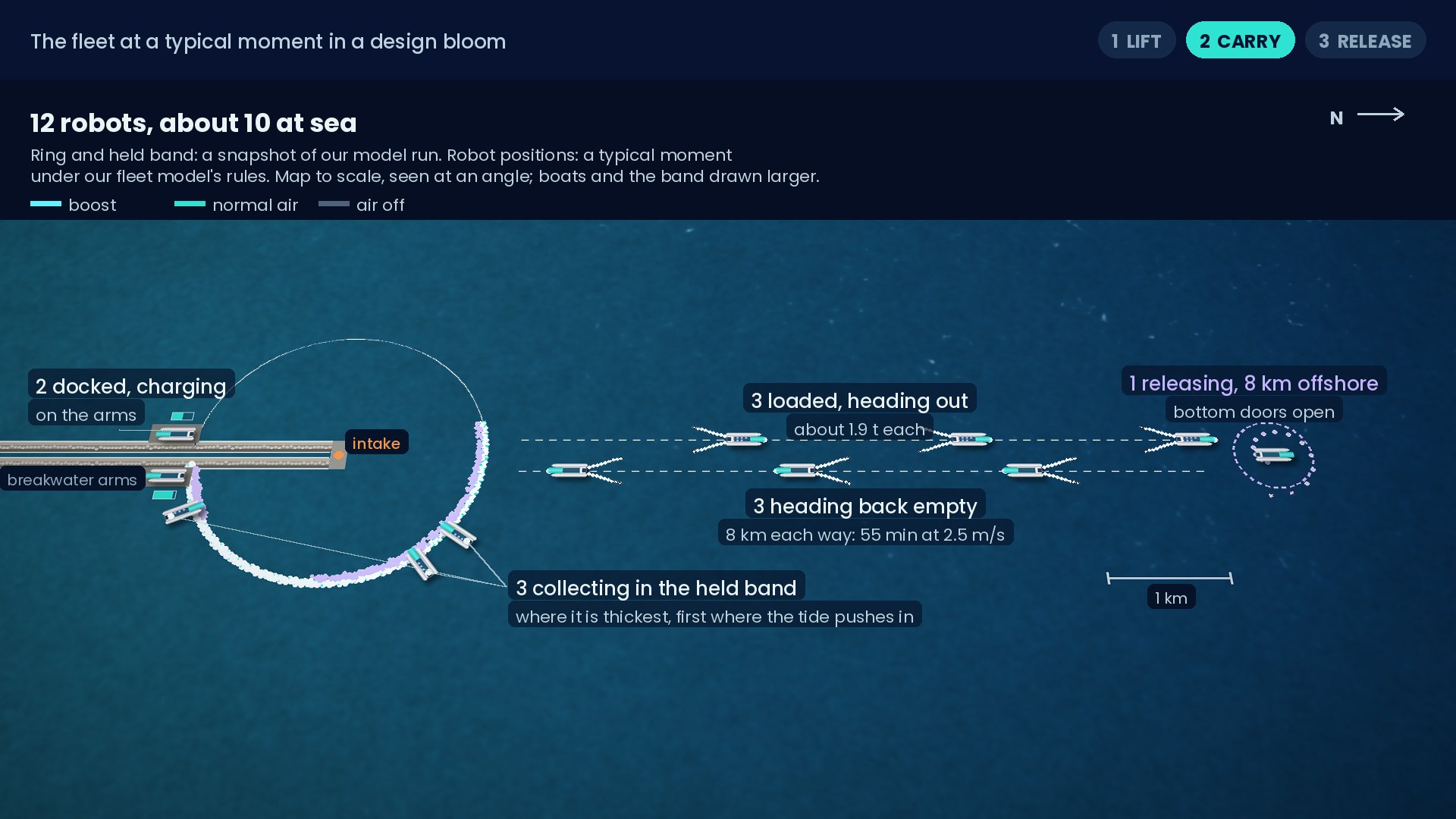
12 robots, about 10 at sea
Each robot works about 7.56 h per charge and then charges for 1.54 h, so it is at sea 0.83 of the time: 12 robots keep about 10 at sea.Show the calculationHide the calculation
working time = trips per charge × trip cycle; charging time = trips per charge × energy per trip ÷ (charger efficiency × charger power) + berthing; availability = working time ÷ (working time + charging time); robots at sea = availability × fleet, rounded
| Input | Value | Source |
|---|---|---|
| Energy per trip cycle | 77.5 kWh | Model output robot_sizing.json |
| Battery; usable share | 300 kWh; 80 % | Our assumption design choice |
| Trips per charge | 3 | Model output robot_sizing.json |
| Trip cycle: collecting + travelling and release | 31 + 120 min | Model output robot_sizing.json |
| Charger; charger efficiency; berthing time | 200 kW; 0.9; 0.25 h | Our assumption design choice |
Working: 3 × 151 min = 7.56 h; charging: 3 × 77.5 kWh ÷ (0.9 × 200 kW) + 0.25 h = 1.29 + 0.25 = 1.54 h
7.56 ÷ (7.56 + 1.54) = 0.831 → 0.83
0.831 × 12 = 10.0 → 10 at sea
The screw: 2.2 m, 21 rpm, 1 m³/s
A 2.2 m Archimedes screw turning at about 21 rpm lifts 1 m³/s of water, with the jellyfish, into the live well: a slow lift. The screw stops if a turtle, dugong or fish is within 5 m. Designed for live handling; survival rates are measured in the Phase 0 trials.Show the calculationHide the calculation
| Input | Value | Source |
|---|---|---|
| Diameter; core; flights; pitch | 2.2; 1.1; 3; 2.2 m | Our assumption design choice |
| Incline; length | 30°; 4.2 m | Our assumption design choice |
| Speed needed; limit for this diameter | 21.3; 29.6 rpm | Model output phase2_Q400.json |
| Tip speed; shaft power | 2.45 m/s; 17.2 kW | Model output phase2_Q400.json |
| Flow; lift | 1 m³/s; 1.2 m | Our assumption design choice |
| Intake mouth diameter at 0.5 m/s | 1.6 m | Model output robot_sizing.json |
| Suction speed 5 m from the mouth | 0.6 cm/s | Model output robot_sizing.json |
| Wildlife stop distance (camera and sonar) | 5 m | Our assumption design choice; tested at sea in step 2 |
21.3 rpm, below the 29.6 rpm limit → about 21 rpm
Trip and fleet rate: about 1.9 t, 55 min each way, 7.2 t/h
Each trip carries about 1.9 t, 55 min each way at 2.5 m/s; in a design bloom the fleet removes 7.2 t/h.Show the calculationHide the calculation
leg time = distance ÷ speed, rounded up to whole 5 minutes; fleet rate = robots at sea × rate per robot in the fleet model
| Input | Value | Source |
|---|---|---|
| Mean distance to the release zone | 8.03 km | Model output release_zone_q400.json |
| Transit speed | 2.5 m/s | Our assumption design choice |
| Trip-sizing stage: load per trip; trip cycle; rate per robot | 1.94 t; 151.2 min; 0.78 t/h | Model output robot_sizing.json |
| Fleet model (12 starts, band model): rate per robot at sea; mean load per trip | 0.724 t/h; 1.90 t | Model output fleet_rates.json |
8.03 km ÷ 2.5 m/s = 53.5 min → 55 min
10 × 0.724 t/h = 7.24 t/h → 7.2 t/h
The two robot numbers come from different model stages: the earlier trip-sizing stage gives about 1.9 t per 151-minute cycle; the fleet model gives the rate per robot used for the whole fleet. Neither is derived from the other.
The robot hull
A battery catamaran: two hulls 12 m long, each 1.4 m wide with a 0.9 m draft, 6.2 m wide overall.Show the calculationHide the calculation
| Input | Value | Source |
|---|---|---|
| Hull length; hull width; draft | 12; 1.4; 0.9 m | Our assumption design choice |
| Overall width | 6.2 m | Our assumption design choice: leaves a gap between the hulls for the live well and the screw tube |
Gap between the hulls: 6.2 − 2 × 1.4 = 3.4 m
3.6 Choosing the fleet
Choosing the fleet: 12 robots, by a fixed decision rule
The decision rule is written into the aggregation code and applied the same way to every fleet. All five fleets are within the 10 % cost band; the 70 % floor leaves 8, 10 and 12 robots tied; the worst-hour tie-break picks 12 (17 cases, against 19 and 21).Show the calculationHide the calculation
- Metric. For each fleet: annualised cost (middle of the low and high estimates) ÷ tonnes kept out of the intake per design bloom, central case.
- Tie band. The best is $147k per tonne (ring + 8 robots). Every fleet within 10 % of it, up to $162k per tonne, is tied: all five are.
- Floor. Keep only fleets with a central reduction of at least 70 %: the ring alone (55.0 %) and 6 robots (67.0 %) drop out.
- Tie-break. Fewest tide-start cases, over all four current cases, whose worst hour exceeds no ring's by more than 2 Poisson standard deviations: 8 robots 21, 10 robots 19, 12 robots 17. 12 robots.
- Second tie-break (not needed): smallest failure pulse.
Swipe sideways to see the whole table.
| Fleet | Annualised, mid ($M/yr) | Kept out per bloom (t) | $k per tonne | Within 10 %? | Reduction | ≥ 70 %? | Worst-hour cases | Failure pulse, central case (t) | Result |
|---|---|---|---|---|---|---|---|---|---|
| Ring, tide-aware air | 18.8 | 120.3 | 156 | yes | 55.0 % | no | 37 | 115 | below the floor |
| Ring + 6 robots | 21.8 | 146.5 | 149 | yes | 67.0 % | no | 24 | 83 | below the floor |
| Ring + 8 robots | 22.8 | 154.8 | 147 | yes | 70.8 % | yes | 21 | 77 | tied |
| Ring + 10 robots | 23.7 | 158.7 | 150 | yes | 72.6 % | yes | 19 | 74 | tied |
| Ring + 12 robots | 24.7 | 164.5 | 150 | yes | 75.3 % | yes | 17 | 69 | picked |
Worst-hour cases are counted over all 96 tide-start cases. Reduction = central case. The failure pulse column is the central case: for 12 robots, 69 t is the central case of the 53–72 t failure pulse in 3.4.
Cost per tonne and worst-hour counts: Model output summary.json. Annualised cost: see 3.9. 8 robots are the cheapest per tonne at both the low and the high cost estimate; the tie-break on peak hours picks 12. One model setting, a cap on how fast spare robot capacity removes held jellyfish, does not scale with fleet size; it could shift how 8, 10 and 12 robots compare and is not yet quantified.
3.7 The 8 km release
Release 8 km offshore: none back within 21 days
Released 8 km offshore, none drift back to the ring within 21 days in our model (at 400 m³/s). Released animals that leave the 16 km model area are not tracked further: none leave with no background current (0 %), 83 % leave with the random current and 100 % with a steady ±0.05 m/s current.Show the calculationHide the calculation
share back = released jellyfish that re-enter the ring within 21 days ÷ all released
Swipe sideways to see the whole table.
| Release distance | No current | Steady +0.05 m/s | Steady −0.05 m/s | Random current | 690 m³/s, no current | Leg time |
|---|---|---|---|---|---|---|
| 5 km | 100 % | 0 % (100 % left) | 0 % (100 % left) | 0 % (83.3 % left) | 100 % | 35 min |
| 8 km | 0 % | 0 % (100 % left) | 0 % (100 % left) | 0 % (83.3 % left) | 13.8 % | 55 min |
| 10 km | 0 % | 0 % (100 % left) | 0 % (100 % left) | 0 % (83.3 % left) | 0 % | 70 min |
Share back at the ring within 21 days; in brackets, the share that left the 16 km model area and was not tracked further (sources: Model output release_zone_q400.json and Model output release_zone_q690.json). With no background current none leave the area and none return from 8 km. At 5 km with no current, all return by day 21 (median 14 days). At 690 m³/s with no current, 13.8 % return from 8 km. Each case: 12 release times × 200 virtual jellyfish.
3.8 Sensing
Sensing: with 16 current meters the result is still 75 %
In the model the controller knows the current at every section. With 16 current meters and a tide forecast instead, the result is 75 % (74.96 % against 75.27 %, same tide starts).Show the calculationHide the calculation
16 meters spread evenly along the ring read the inward speed with 0.01 m/s noise; a tide-and-intake prediction fills in between them. Same seeds and tide starts as the main runs; results compared start by start.
| Input | Value | Source |
|---|---|---|
| Intake per tide start, with the meters | 24 values | Model output _s16rand_s00–s23.json |
| Intake per tide start, full knowledge | 24 values | Model output rand_s00–s23.json |
Reduction 74.96 % against 75.27 %: −0.32 ± 0.53 points (paired 2 SE); 8 starts worse, 10 better, 6 equal
Share reaching 3.84 % (against 3.79 %); 18.2 t/day (against 18.0); tide-aware air alone 54.3 % (against 55.0 %)
The bound cases (Shamal, offshore wind, design-maximum flow) use the same full-knowledge controller.
3.9 Cost
Build cost: $102–252M
$102–252M to build, a class-5 early estimate (±50 %).Show the calculationHide the calculation
CAPEX = direct cost × (1 + engineering and management) × (1 + contingency)
| Line | Quantity | $M, low–high |
|---|---|---|
| Blowers, 400 kW turbo, one plant on both arms | 44 units, 17.6 MW | 26.4–52.8 |
| Seawater aftercoolers to 40 °C, pumps | 17.4 MW heat | 1.6–7.5 |
| Deep main DN1600, ballast SF 1.5 | 7,692 m | 15.2–34.6 |
| Shallow main DN1200, ballast SF 1.5 | 2,519 m | 3.5–8.6 |
| Channel crossing DN1600, buried | 250 m | 0.7–1.7 |
| Diffusers 4 × DN110 | 30,767 m | 1.0–3.7 |
| 60 air-piloted pinch valves DN400, float-line control boxes, DN300 sub-header | 60 | 1.3–3.3 |
| Float line with 1.5 m mesh skirt (passes ≥ 90 % of flow) | 7,656 m | 1.1–4.6 |
| Moorings, double legs every 50 m | 308 | 1.5–4.6 |
| Current meters (ADCP) | 16 | 0.6–1.3 |
| SCADA, comms, software | 1 lot | 1.0–3.0 |
| Relocation robots | 12 | 12.0–30.0 |
| Docks, 6 berths each | 2 | 2.4–6.0 |
| Direct cost | 68.5–161.6 | |
| Engineering and management (EPCM), 15–20 % | 10.3–32.3 | |
| Contingency, 30 % | 23.6–58.2 | |
| Build cost (CAPEX) | 102.3–252.2 |
| Input | Value | Source |
|---|---|---|
| Line items and quantities | 13 lines | Model output cost2_r12.json |
| Unit prices | low–high | Our assumption class-5 unit prices, not verified against quotes |
Low: 68.5 × 1.15 × 1.30 = 102.3; high: 161.6 × 1.20 × 1.30 = 252.2 ($M)
→ $102–252M
Running cost: $2.6–13.2M a year
$2.6–13.2M a year: energy for 30–90 days a year on, plus maintenance.Show the calculationHide the calculation
running cost = energy per day × days on × electricity price + maintenance (share of CAPEX)
| Input | Value | Source |
|---|---|---|
| Energy per day, air and robot charging | 345 MWh | Model output cost2_r12.json |
| Days on per year (low / high) | 30–90 | Our assumption the ring runs only in the bloom season |
| Electricity price (low / high) | $54–100/MWh | Published ADDC 2025 |
| Maintenance (low / high) | 2–4 % of CAPEX a year | Our assumption planning allowance, not a quote |
Low: 344.5 MWh × 30 days × $54/MWh = $0.56M, plus 2 % × $102.3M = $2.05M: total $2.60M
High: 344.5 MWh × 90 days × $100/MWh = $3.10M, plus 4 % × $252.2M = $10.09M: total $13.19M
→ $2.6–13.2M a year
Annualised cost: $12.3–37.2M a year
$12.3–37.2M a year: the build cost spread over the equipment's life at 8 % interest, plus the running cost.Show the calculationHide the calculation
CRF(i, n) = i ÷ (1 − (1 + i)−n); annualised = (CAPEX − robots and docks) × CRF(8 %, 30 yr) + robots and docks × CRF(8 %, 15 yr) + running cost
| Input | Value | Source |
|---|---|---|
| Interest rate | 8 % | Our assumption cost of capital for a utility project |
| Life: ring and air plant / robots and docks | 30 / 15 years | Our assumption robots and docks wear out sooner |
| Robots and docks, with engineering and contingency | $21.53–56.16M | Model output cost2_r12.json |
| CAPEX; running cost | $102.3–252.2M; $2.60–13.19M/yr | Model output cost2_r12.json |
CRF(8 %, 30) = 0.0888; CRF(8 %, 15) = 0.1168
Low: 80.81 × 0.0888 + 21.53 × 0.1168 + 2.60 = 12.30
High: 196.01 × 0.0888 + 56.16 × 0.1168 + 13.19 = 37.16
→ $12.3–37.2M a year
Break-even: 4–20 lost unit-days a year
TAWQ pays for itself if it avoids 4–20 lost unit-days a year (one reactor unit offline for one day), with electricity valued at $54–100/MWh: Abu Dhabi business tariffs used as a proxy, because Barakah's sale price is not public.Show the calculationHide the calculation
value of one unit-day = unit size × 24 h × price; break-even = annualised cost ÷ value of one unit-day
| Input | Value | Source |
|---|---|---|
| Unit size | 1,400 MW | Published Power Engineering 2021 |
| ADDC business tariffs, 2025 | 20–36.6 fils/kWh | Published ADDC 2025 |
| Dirham to US dollar | 3.6725 AED per US$ | Published CBUAE 2014 |
| Annualised cost (low / high) | $12.30–37.16M | Model output summary.json |
Price: 20–36.6 fils/kWh = 200–366 AED/MWh; ÷ 3.6725 = $54.46–99.66/MWh → $54–100/MWh
One unit-day: 1,400 MW × 24 h × $54–100/MWh = $1.81–3.36M
Fewest: $12.30M ÷ $3.36M = 3.7; most: $37.16M ÷ $1.81M = 20.5
3.7–20.5 → 4–20 lost unit-days a year
For scale: one bloom at Gravelines took four units offline at once. We do not claim a number of avoided shutdowns.
3.10 Phase 0 sample size
Phase 0 sample size: 100 animals per arm
100 animals per arm are enough to tell 90 % survival from 75 %.Show the calculationHide the calculation
n = (z1−α/2 √(2 p̄ (1 − p̄)) + z1−β √(p₁(1 − p₁) + p₂(1 − p₂)))² ÷ (p₁ − p₂)²
| Input | Value | Source |
|---|---|---|
| Pass mark p₁; rate to rule out p₂ | 90 %; 75 % | Our assumption the pass gate and the lowest survival we must be able to detect |
| Two-sided α; power | 0.05; 80 % | Our assumption standard choices |
| Stored sample size | 100 | Model output phase2_spec.json |
n = 99.5 → 100 per arm
Assumptions, and how they will be tested
In shortWhat the results rest on: which parts are published, which our models computed, which we assumed, and how each will be tested if we are shortlisted.
If shortlisted: three gated steps
Phase 0 survival trials (bubbles, mesh, screw, full chain; 100 animals per arm). (indicative: one bloom season, our assumption, since live jellyfish are needed)
Gate≥ 90 % full-chain survival
Animals held at the curtain are scored too: bubbles can harm medusae larger than 3 cm (Raskoff et al. 2003), and the field trial of a bubble curtain did not measure injury (Haberlin et al. 2021).
100 m pilot section + 1 robot at sea (holding, sliding, fouling, capture rate, wildlife stop). (indicative: one bloom season)
Gateholding ≥ modelled limit; mesh ≤ 10 % blocked
Full ring + 12 robots, with mooring and storm loads designed.
GateFANR and EAD approvals
Phase 0 is step 1, the survival trials.
Assumption register
| Assumption | Value | Basis | How it will be tested |
|---|---|---|---|
| Design bloom | 5 g/m³ (about 1,400 t within 4 km)No published Gulf biomass density was found. | Our assumption | Not field-tested: a design case |
| Dense bloom (stress test) | 30 g/m³ | Our assumption | Not field-tested: a stress case |
| Intake flow | 400 m³/s (bound 690)Condenser flow only; safety-related essential service water has its own “essential service water intake structure” (FANR 2012). | Published ENEC 2017 · NEI 2012 · FANR 2012 | Not needed: published |
| Jellyfish movement | drift with the water; held ones slide along the curtainSwimming is not modelled. | Our assumption | Step 2: sliding along the curtain at the pilot section |
| Mesh skirt blocked | 10 %At 40 % blocked, holding collapses; the fouling rate is unknown. | Our assumption | Step 2: fouling rate; gate: mesh ≤ 10 % blocked |
| Hold-time basis | 12 h | Our assumption | Step 2: holding at the pilot section |
| Holding factors (mesh + 12-h hold) | ×0.85 normal air, ×0.76 boostTyped into the model; they reproduce from the curtain-model runs: 0.904 × 0.943 and 0.801 × 0.943. | Model output | Step 2: holding; gate: holding ≥ the modelled limit |
| Holding limits | 0.081–0.112 m/s normal; 0.085–0.126 m/s boost | Model output | Step 2: holding; gate: holding ≥ the modelled limit |
| Background current | random: σ 4.8 cm/s, τ 2 days; bounds: steady 0, ±0.05 m/sσ is the spread between measured currents and the tide-only reconstruction, “a relatively large influence of non-tidal forcing”; τ has no source. | σ: Published (Nesterov et al. 2023); τ: Our assumption | Not field-tested |
| Shamal case | steady 10 m/sReal Shamals: 15–20 m/s for 24–36 hours or 3–5 days (Thoppil & Hogan 2010); not modelled. | Our assumption Thoppil & Hogan 2010 | Not field-tested |
| Sensing | 16 current meters + 10-min tide forecast; modelled with full knowledge of the currentWith the meters and forecast: 75 % (74.96 against 75.27 %, same starts). | Model output | Not field-tested (checked in the model) |
| Air control rules | off if forecast inward < −0.02 m/s; boost if > 0.8 × limit; power capped at 14.63 MW | Our assumption (design rule) | Not field-tested (design choice) |
| Robot availability | 0.83 (12 robots → about 10 at sea)Round(0.83 × 12) = 10. | Model output | Step 2: one robot at sea |
| Robot trip | about 1.9 t per trip, 2.5 m/s, 55 min each way | Load and leg time: Model output; speed: Our assumption | Step 2: capture rate at sea |
| Wildlife stop | screw stops if an animal is within 5 mUntested. | Our assumption (design rule) | Step 2: wildlife stop at sea |
| Release | 8 km offshore: none back within 21 daysAt 400 m³/s. With a steady or random current most releases leave the model area; at 690 m³/s with no current, 13.8 % return. | Model output | Not field-tested (model result); step 1, the Phase 0 survival trials, measures survival through the full chain |
| Failure pulse | an estimated 53–72 t if the air fails at maximum held stockThe share comes from leaked animals, not a simulated band release. | Model output (proxy) | Not field-tested (model estimate) |
| Mouth speed | about 0.38 m/s (area 1,053 m² = 162 m × 6.5 m)Width fitted to NMDC's area; a 7.0 m depth would give 0.35 m/s. | Model output (estimate) NMDC | Not field-tested (estimate) |
| Electricity value | $54–100/MWhBarakah's sale price is not public. | Published (proxy) ADDC 2025 | Not tested (economic input) |
| Cost estimate | class 5, ±50 %Unit prices not verified. | Our assumption | Not tested; refined as the design develops |
| Finance | 8 % interest; 30-year life (robots, docks 15 years) | Our assumption | Not tested (economic input) |
| Running period | 30–90 days a year; maintenance 2–4 % of CAPEX a year | Our assumption | Not field-tested |
| Plant | 4 units × 1.4 GW = 5,600 MW | Published Power Engineering 2021 | Not needed: published |
| Seabed profile and channel lengths | One transect read from the ETOPO 2022 global relief model, not survey data; the three channels 14.50 km long in totalAdded on this site; not in the deck's assumption table. NMDC publishes no channel widths or lengths. | Our assumption ETOPO 2022 · NMDC | Not field-tested |
The robots are designed for live handling; survival rates are measured in the Phase 0 trials.
Options rejected and why
In shortWe tried the obvious answers first; each one fails for a reason our models or simple physics show.
Bigger screens, faster washing
Treats the symptom: the same tonnes still reach the plant, and the animals still die on the screens.
→ Load unchanged
A net across the mouth
Catches the same tonnes one step earlier. Nets clog and can entangle turtles and fish.
→ Load moved, not removed
A bubble curtain at the mouth
Water there moves at about 0.38 m/s. A bubble curtain holds against at most about 0.13 m/s.
→ Holds nothing
One straight curtain offshore
Our site flow model found no reliable current direction at the site, so an open line is outflanked when the tide turns.
→ It has to be a closed ring
Fixed air on the ring
With fixed air, 80.4 % of the jellyfish drifting in meet a section that can hold them, against 86.9 % with tide-aware air, and 8.8 % of the bloom reaches the intake against 6.9 %. Tide-aware air also uses 12 % less power.
→ Replaced by tide-aware air
Release at 5 km
With no background current, all released jellyfish came back to the ring by day 21 (median 14 days); from 8 km, none did.
→ Release at 8 km
Releasing downstream instead of straight offshore
No gain in the release model: the background current reverses within days.
→ Straight offshore
A smaller fleet
The ring alone (55 %) and 6 robots (67 %) miss the 70 % floor; 8 and 10 robots have more worst-hour cases (21 and 19, against 17).
→ 12 robots
How we verified
In shortWe re-ran the models from scratch and traced every published number back to the file it came from: the results reproduce.
We re-ran the models
175 of 179
result files came out bit-for-bit identical
The whole final stage (four current cases × 24 tide starts, the bound cases and the dense bloom) was re-run from scratch on 10 Oct 2026 on a different computer (Windows instead of Linux, same library versions). The other four files differ only by last-digit rounding, one dense-bloom value that no document quotes, and three hand edits that no script makes: the robot payload typed as 1.9 t instead of the computed 1.94 t, a cycle-time field removed, and a note on the 240-valve loss added. The headline is identical to every digit, and so are the fleet decision and the 17 of 96 worst-hour count.
We traced every number
191
numbers traced to the result files
Every number in our deck, video draft, platform texts and internal team document was traced to the file it came from and re-derived: 151 traced and rounded correctly; 8 were correct but needed a qualifier; 11 were external facts, checked against sources; 10 were design inputs; and 6 wording issues, 3 mismatches, 1 rounding issue and 1 title item were found and corrected before submission (191 in all).
We checked the code
15 of 20
claims match the code
We checked 20 claims against the code: 15 match, 3 match in part and 2 did not. All of them are disclosed on this page: the controller's full knowledge of the current (checked with current meters), the convergence check (the first half of the tide starts against all of them, within 5 %), which fails in two steady-current cases (below), the typed-in holding factors (reproduced), the failure-pulse proxy (3.4) and the fitted channel width (3.1).
The convergence check, stated plainly
Before the runs we set a check: the total intake over the first 12 tide starts should agree with all 24 within 5 %. It passes in the central case (no ring +4.8 %, ring + 12 robots +3.4 %). In two steady-current bound cases for 12 robots it does not: −14.9 % at 0 m/s, on a small 0.68 % share, and +5.7 % at −0.05 m/s. Those two steady-current results are less settled than the central case.
| Configuration | Central | Steady 0 | Steady +0.05 | Steady −0.05 |
|---|---|---|---|---|
| No ring | +4.8 % passes | −0.4 % passes | −0.2 % passes | +1.3 % passes |
| Ring + 12 robots | +3.4 % passes | −14.9 % fails | −3.9 % passes | +5.7 % fails |
This page itself is built by a script from the final result files, and an automatic check compares each number and its rounding with our proposal deck.
References
In shortThe published sources we used, with the sentence each one supports and working links.
ENEC (2026). Challenge statement, Advanced Technology Pioneers 2026, on the ChallengeON platform.
https://challengeon.atrc.ae/en/challenges/atp2026/pages/enec-challenge-statement?lang=en
Supports: The problem statement, the scope (after an early-warning notification), the focus species, the data rule and the AI-use rule. Accessed 10 Oct 2026.
“Problem Statement: HOW MIGHT WE ADVANCE THE SUSTAINABLE MANAGEMENT OF SEASONAL JELLYFISH BLOOMS IN COASTAL ENVIRONMENTS?” “The challenge focuses on sustainable jellyfish management after an early-warning notification.”
ENEC (7 Feb 2017). Final Condenser for the Barakah Nuclear Energy Plant… (news release).
Supports: Condenser cooling-water flow of about 6,000 m³ per minute per unit. Accessed 10 Oct 2026.
“…will have a volume of 6000 m3 of sea water per minute passing through them…”
Power Engineering, R. Walton (7 Apr 2021). Barakah, first nuclear power plant in UAE, starts commercial operations.
Supports: Unit size 1.4 GW; four units, 5,600 MW. Accessed 10 Oct 2026.
“…full connected stage for 1.4-GW Unit 1” “Barakah's four units eventually will generate 5,600 MW at full capacity”
Nuclear Engineering International (28 Sep 2012). Building Barakah.
https://www.neimagazine.com/advanced-reactorsfusion/building-barakah/
Supports: Design maximum cooling-water flow of 172.5 m³/s per unit (our 690 m³/s bound). Accessed 10 Oct 2026.
“…with a maximum flow rate of 172.5 m3/second/unit.”
FANR (2012). Safety Evaluation Report (summary) of an application for a licence to construct Barakah Units 1 and 2.
Supports: Safety-related essential service water uses Gulf seawater through its own intake structure, so 400 m³/s is the condenser flow only. Accessed 10 Oct 2026.
“The ESW system utilizes water from the Arabian Gulf (the plant UHS) to remove heat from plant SSCs.” “…essential service water intake structure HVAC, and circulating water intake structure HVAC systems…”
NMDC Group. Barakah NPP marine works (project page).
https://nmdc-group.com/en/dredging-and-marine/barakah-npp-marine-works/
Supports: Total dredged area of the three channels, 2.35 km², and their depths; no channel widths are published. Accessed 10 Oct 2026.
“…dredging of an intake channel for cooling water intake, discharge channel for hot water release and a navigation channel for wharf access.” “The total area dredged was approximately 2.35Km2 at the final depth of the channels, which range from -5.5 MSL to --9.5 [sic] MSL.”
NOAA National Centers for Environmental Information (2022). ETOPO 2022 15 Arc-Second Global Relief Model.
https://doi.org/10.25921/fd45-gt74
Supports: The seabed depth profile in our site model (one transect, read from this global relief model; not survey data), which sets the ring depths and the channel lengths. Accessed 10 Oct 2026.
Nesterov, O. et al. (2023). A numerical assessment of the dispersion of dissolved pollutants in the Arabian Gulf associated with the Barakah nuclear power plant. Ocean Modelling 186, 102274.
https://doi.org/10.1016/j.ocemod.2023.102274
Supports: Spread of the non-tidal (background) current, 4.8 cm/s. Accessed 10 Oct 2026.
“...[RMSE] between the measured current velocities and those reconstructed from the tidal harmonics is 4.8 cm/s with the correlation coefficient of 50.1%. This indicates a relatively large influence of non-tidal forcing.”
Thoppil, P. G. and Hogan, P. J. (2010). Persian Gulf response to a wintertime shamal wind event. Deep-Sea Research I 57(8), 946–955.
https://www7320.nrlssc.navy.mil/pubs/2010/prasad1-2010.pdf
Supports: Real Shamal winds typically reach 15–20 m/s and last 24–36 hours or 3–5 days. Accessed 10 Oct 2026.
“Based on duration, there are two types of winter shamal: those which last 24–36 h and those which last for a longer period of 3–5 days. During a shamal, winds typically reach 15–20 m s−1 near the surface during the daytime.”
Abu Dhabi Distribution Company (ADDC). Rates and tariffs 2025, business customers.
https://www.addc.ae/en-US/business/Pages/RatesAndTariffs2025.aspx
Supports: Business electricity tariffs of 20–36.6 fils/kWh, used as a proxy for the value of lost output. Accessed 10 Oct 2026.
“Electricity 20 fils For 1 kWh” “27 fils … 36.6 fils For 1 kWh”
Central Bank of the UAE. Annual Report 2014, Chapter 5, p. 39.
https://www.centralbank.ae/media/e44dkkze/cbuae-annual-report-2014-en.pdf
Supports: The dirham's fixed rate of 3.6725 per US dollar, used to convert ADDC's tariffs to US dollars. Accessed 10 Oct 2026.
“The fixed peg of the exchange rate of the dirham to the US dollar, at a rate of 3.6725 dirhams per US dollar, means that the CBUAE has limited degree of freedom to set interest rates…”
AFP, via L'info durable (13 Aug 2025). Méduses à la centrale nucléaire de Gravelines : un premier réacteur a redémarré (in French).
Supports: Jellyfish shut down Gravelines units 2, 3, 4 and 6 on 10–11 Aug 2025. Accessed 10 Oct 2026.
“Les unités de production n°2, 3 et 4, arrêtées automatiquement depuis dimanche soir pour la même raison” “Le réacteur n°6 a redémarré ce matin à 7H30”
Raskoff, K. A., Sommer, F. A., Hamner, W. M. and Cross, K. M. (2003). Collection and culture techniques for gelatinous zooplankton. Biological Bulletin 204(1), 68–80.
https://doi.org/10.2307/1543497
Supports: Air bubbles can harm medusae larger than 3 cm, so Phase 0 scores animals held at the curtain. Accessed 10 Oct 2026.
“Although air bubbles can be helpful in the culture of many small gelatinous animals by increasing water circulation, they can be detrimental to larger adult sizes (>3 cm).”
Haberlin, D., McAllen, R. and Doyle, T. K. (2021). Field and flume tank experiments investigating the efficacy of a bubble curtain to keep harmful jellyfish out of finfish pens. Aquaculture 531, 735915.
https://doi.org/10.1016/j.aquaculture.2020.735915
Supports: A high-airflow bubble curtain deflected large jellyfish in the field; the study reports no injury or survival data. Accessed 10 Oct 2026.
“a high air flow 8 m linear bubble curtain set at 5 m depth effectively deflected large compass jellyfish” “increased wave height and increased air flow increased jellyfish transport through the curtain”
AI use
In shortHow we used AI, in the words on our proposal deck.
AI use: we used Claude (Anthropic) to help write, debug and run our simulation code, check sources, and draft figures, slides and illustrations. The team set the methodology, made the design decisions, and interpreted the results.
The team · Mechanical & Mechatronics Engineering · HCT Dubai
Sifana Habtamu · Amanuel Mulugeta · Abel Bekele · Sara Khalid Ali Maleeh Alshamsi
Model code: available on request.
Glossary
- Bubble curtain
- A line of seabed pipes releasing air. The rising bubbles drive a surface current that pushes drifting jellyfish back.
- Holding limit
- The fastest inward water speed a bubble curtain can still hold jellyfish against.
- Tide-aware air
- Air that is boosted where the tide pushes water in and switched off where it flows out.
- Design bloom
- Our 3‑day test bloom: 5 g of jellyfish per m³ of water, about 1,400 t within 4 km of the intake. Dense bloom: 30 g/m³.
- Central case
- The model run with a randomly varying background current. Steady currents of 0 and ±0.05 m/s are the bounds.
- Tide start
- When the bloom arrives in the tide cycle. We use 24, spread over one spring–neap cycle.
- Virtual jellyfish
- A computer particle standing for about 119 kg of jellyfish in the design bloom.
- Worst hour
- The largest load reaching the intake in any single hour of the bloom.
- Failure pulse
- What reaches the intake if the air fails when the ring holds the most jellyfish.
- Unit-day
- One reactor unit (1.4 GW) offline for one day.
- CAPEX, running cost
- The one-off build cost; the yearly cost of energy and maintenance.
- Early (class-5) estimate
- A cost estimate made before detailed design, here taken as ±50 %.
- CRF
- Capital recovery factor: turns a build cost into an equal yearly payment over the equipment's life.
- 2 standard errors
- The range the result would likely stay within if the 24 tide starts were drawn again.
- Poisson standard deviation
- The natural scatter of a random count; used to judge whether a worse hour is more than chance.
- Nm³/min
- Cubic metres of air per minute at standard conditions.
- Current meter (ADCP)
- An instrument that measures water speed.
- Phase 0
- The survival trials: step 1 of our three gated steps if shortlisted. Step 2 is a 100 m pilot section with one robot at sea; step 3 the full ring after approvals.
- Live well
- The robot's flooded tank: the jellyfish ride in seawater that flows through it.
- Spring–neap cycle
- The roughly two-week cycle from strong (spring) to weak (neap) tides and back; our tide starts are spread over one cycle (14.77 days).
- Shamal
- A strong seasonal wind over the Gulf. Real Shamals typically reach 15–20 m/s (Thoppil & Hogan 2010).
- Medusa, medusae
- The free-swimming, bell-shaped form of a jellyfish; medusae is the plural.
- Plume
- The column of rising bubbles and water above a bubble pipe; at the surface it spreads into the current that holds jellyfish back.
- Aftercooler
- A heat exchanger that cools the hot air from the blowers before it enters the plastic pipes; ours use seawater.
- σ and τ
- The spread (σ, 4.8 cm/s) and the memory (τ, 2 days: how long a pattern tends to last) of the randomly varying background current in the central case.
- Jackknife
- A way to estimate uncertainty: recompute the result with one tide start left out at a time and see how much it moves.
- ENEC
- Emirates Nuclear Energy Company, which set this challenge.
- ATP
- Advanced Technology Pioneers 2026, the competition this entry is for, run on the ChallengeON platform.
- FANR
- Federal Authority for Nuclear Regulation, the UAE's nuclear regulator.
- EAD
- Environment Agency – Abu Dhabi.
- SCADA
- Supervisory control and data acquisition: the computer system that monitors and controls the air plant and valves.
- DN
- Diameter nominal: the standard size code of a pipe, in millimetres.